For this project, we will be simulating the 2D steady-state incompressible flow over the NACA 25-209 airfoil profile at 𝑅𝑒 = 3.0 × 10⁶ using OpenFOAM. Furthermore, the effect of the angle of attack on the force coefficients will be investigated. The angles of attack that are of our interest are {−5°, 0°, 5°, 10°}. For consistency, the boundary conditions, the turbulence model, the solver, and the tolerances for all the angles of attacks were kept the same.
Boundary Conditions
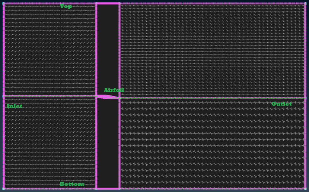
Boundary conditions that were used during this experiment were of Neumann and Dirichlet types. To construct a Neumann Boundary Condition, one must provide the flux at that boundary. Note that the actual value at that boundary is unknown. Moreover, to construct a Dirichlet Boundary Condition, one must provide a fixed value for that specific boundary. Refer to figure 1 to understand where each boundary is located. additionally, Tables 1 to 4 provides the boundary conditions used during this experiment.
Figure 1: Boundary locations
Table 1: Velocity boundary conditions and types
Boundary Locations
Boundary Value
Boundary Type
Inlet
Freestream at 44.1 𝑚/𝑠 in +x
direction
Dirichlet
Outlet
Freestream at 44.1 𝑚/𝑠 in +x
direction
Dirichlet
Top and Bottom
No Slip
Dirichlet
Airfoil
No Slip
Dirichlet
Front and Back
Empty
None
Table 2: Pressure boundary conditions and their types
Boundary Locations
Boundary Value
Boundary Type
Inlet
Zero gradient
Neumann
Outlet
Freestream Pressure at
0 𝑚2
/𝑠
2
Dirichlet
Top and Bottom
Zero gradient
Neumann
Airfoil
Zero gradient
Neumann
Front and Back
Empty
None
Table 3: Nut boundary conditions and their types
Boundary Locations
Boundary Value
Boundary Type
Inlet
Freestream at
1.470 × 10⁻⁵ 𝑚2
/𝑠
Dirichlet
Outlet
Freestream at
1.470 × 10⁻⁵ 𝑚2
/𝑠
Dirichlet
Top and Bottom
nutUSpaldingWallFunction at
a value of 0
Dirichlet
Airfoil
nutUSpaldingWallFunction at
a value of 0
Dirichlet
Front and Back
Empty
None
Table 4: NuTilda boundary conditions and their types
Boundary Locations
Boundary Value
Boundary Type
Inlet
Freestream at
5.88 × 10⁻⁵ 𝑚2
/𝑠
Dirichlet
Outlet
Freestream at
5.88 × 10⁻⁵ 𝑚2
/𝑠
Dirichlet
Top and Bottom
Fixed value of 0 𝑚2
/s
Dirichlet
Airfoil
Fixed value of 0 𝑚2
/s
Dirichlet
Front and Back
Empty
None
The free stream velocity of 44.1 𝑚/𝑠 was chosen to match the requested Reynolds number and the properties of air. The following equation was used to calculate the velocity value:
𝑅𝑒 = 𝑈𝐶/𝑣
Where: Re is the Reynolds number and is 3.0 × 10⁶ 𝑣 is the kinematic viscosity of air and is 1.470 10−5 𝑚2/𝑠 𝐶 is the chord length and is 1 𝑚
The initial values for turbulent kinetic viscosity (nut) and the modified turbulent kinetic viscosity (nuTilda) were guessed. However, it was found by trial and error that the solutions are most stable when the value of nuTilda is four times the value of nut and the value of nut is set to 1.470 10−5 𝑚2/𝑠. This value is the kinematic viscosity of the fluid.
Solver and Turbulent model
SimpleFOAM was used as the solver. This solver is used for steady-state cases. Since we are modeling the steady-state flow over the airfoil it would be best to use this solver. Through trial and error, it was found that a relaxation factor of 𝜔𝑈 = 𝜔𝑛𝑢𝑇𝑖𝑙𝑑𝑎 = 0.7 𝑎𝑛𝑑 𝜔𝑃 = 0.3 would make the simulation more stable. Furthermore, the Reynolds Averaged Navier Stokes (RANS) model was used to model the flow. RANS is basically the time-averaged equation of motion for fluid flow. In simple terms, RANS is a decomposition where an instantaneous quantity is decomposed into its time average and its fluctuating parts. Note that the Spalart-Allmaras turbulence model was used to model the Reynolds stress tensor. Spalart-Allmaras is a, one equation linear eddy viscosity model. Many different turbulence models such as k-omega SST and k-epsilon model were tested. However, it was found through trial and error that the Spalart-Allmaras turbulence model was the most stable model.
Y+ Value
It is important to note that wall functions were used to model the turbulence behavior near the walls including the airfoil. A wall function is used when one would like to extend the log layer to the walls. This would imply that the 𝑌+ value must be between 30 and 800. The 𝑌+ calculator on ANSA was used to calculate the estimated minimum first layer height. At a 𝑌+ value of 30, the estimated minimum height was 0.52 mm and at a 𝑌+ value of 800, the estimated first height was 14 mm. The mesh was selected so that the first layer would have a height of 11 mm.Many different types of structured meshes were used. However, after trial and error, it was found that the simple 2D structured mesh would converge faster and is more stable. C-type mesh would fail to converge due to the large amount of non-orthogonality in the mesh. Furthermore, the simple structured mesh with uneven spacing would fail due to the large aspect ratio. Therefore, the simple 2D mesh with no special features was selected.
Domain Sensitivity
Before any simulations could be executed, a domain size must be picked. It is important to note that if the domain size is too small, then the effects of the boundary conditions will propagate inwards and affect the results. If the domain size is too large, then the computational cost would increase dramatically. To find the right domain size four different domain sizes were selected. The element size for all four domains was set to be the same. Then simulations were executed on each of the four domains and the values of 𝐶𝑙 and 𝐶d for each domain were collected. The values of 𝐶𝑙 and 𝐶d that were collected for the domain sensitivity study are not the correct 𝐶𝑙 and 𝐶d values for the airfoil. However, since the element size was constant these values in theory would stop fluctuating at a specific domain size. At this point, one can conclude that the boundaries are not affecting the results. Figure 2 illustrates the dimensions that were changed during the domain size sensitivity test. Additionally, the domain size values for the four runs are listed in table 5. Furthermore, figure 3 shows the variation of 𝐶𝑙 as a function of domain size. As one can observe there are minute differences between run 3 and run four. To be on the safer side domain size four was chosen.
Table 5: The domain size values for the four different domains as a function of chord length C.
Dimensions
Domain 1
Domain 2
Domain 3
Domain 4
Width
0.5C
1C
2C
4C
Up-Stream
0.5C
1C
2C
4C
Down-Stream
1C
2C
4C
8C
Figure 2: Variable dimensions during domain sensitivity analysis
Figure 3: Variation of 𝐶𝑙 as a function of domain size
GCI Study
Before any simulation can be run. One must show that the mesh size will not affect the results of the solution. This can be done by conducting and calculating the Grid Convergence Index (GCI). The GCI is a measure of the percentage, the computed value is away from the asymptotic value. In simple terminology, it indicates how far the solution of the simulation is from the true (asymptotic) value. To conduct a GCI, one must create three different meshes for the same problem. These meshes are all identical in geometry, but they have different resolutions. Table 6 provides the mesh resolution of the three different sizes of mesh that were used (coarse, medium, and fine) for calculating the GCI. At each of the refinements, the 𝐶𝑙 value was extracted and plotted against each other in figure 4. Furthermore, the %GCI values were also plotted in figure 5.
Table 6: number of mesh elements at each size.
Mesh Size
Number of Elements
Coarse
30976
Medium
122500
Fine
490000
Figure 4: Lift coefficient values at different mesh refinements
Figure 5: %GCI of the lift coefficients for the different mesh refinements
As one can see there is a great difference between the finest mesh and the extrapolated value. Furthermore, The GCI provided in figure 5, is still not as good as it should be because we are still far away from the asymptotic range.
To see if we are in the asymptotic range we can use the following equation:
𝐺𝐶𝐼32/(𝑟𝑝 × 𝐺𝐶𝐼21) ≅ 1
Where: 𝑟 is the refinement ratio and is 2 𝑝 is the apparent order and is 1.3549 Plugging the values into the equation we would get:
(18.06/21.3549 × 29.32) ≅ 1
Which would yield:
0.2408 ≠ 1
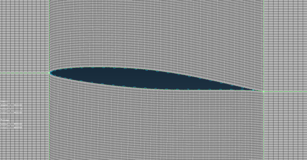
This implies that the mesh must be refined even more. However, at this stage, my computer was not powerful enough to handle the more refined meshes and would crash. Therefore, I decided to pick the finest mesh and work with that. Figure 6 and 7 show the mesh that was selected after the GCI analysis was done.
Figure 6: Selected mesh after GCI analysis.
Figure 7: Zoomed in view of the selected mesh after GCI analysis (Note that the mesh is a structured mesh)
Force Coefficients at different angles of attack
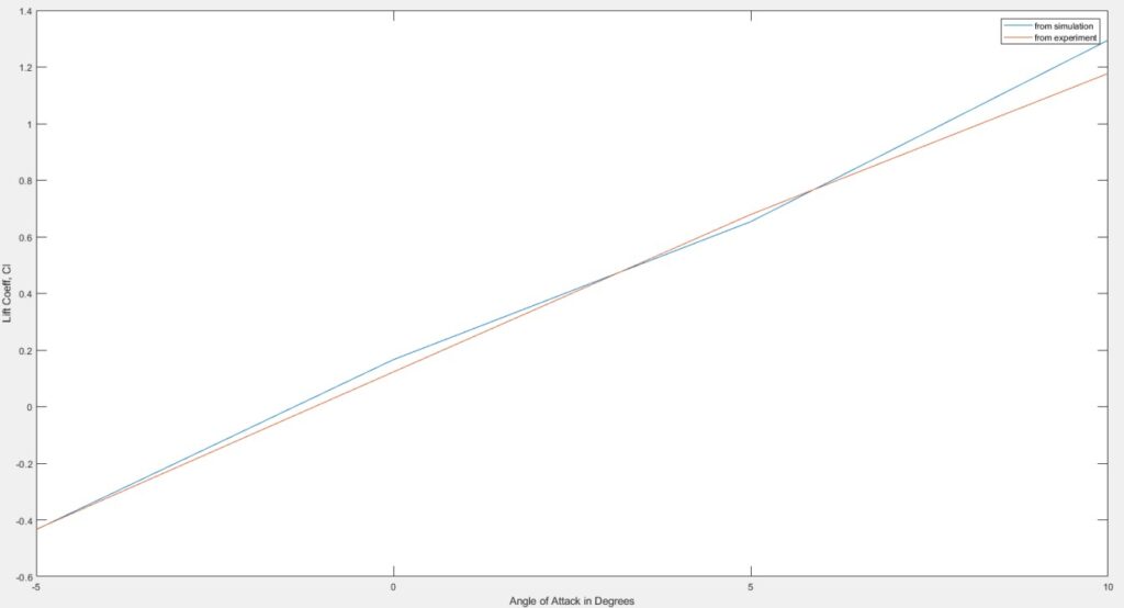
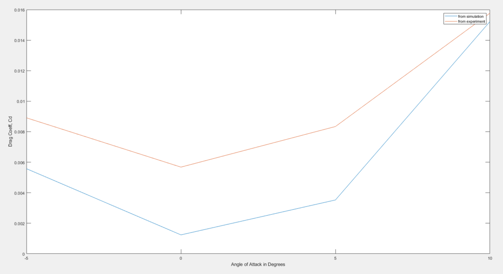
Force coefficients were computed using OpenFOAM and plotted against the experimental data that was found in the (Abbott and Doenhoff, 1959) book. The experimental lift and the simulation lift coefficients agree with each other to a great extent. However, the values of drag coefficients are significantly off. This is mainly due to the fact that drag is composed of multiple components. Drag can be induced due to surface friction, project area, and downstream vortices. The OpenFOAM simulation was set to capture the drag due to the projected area. Therefore, the simulation drag at each angle of attack is off by a significant value. Furthermore, since the drag being calculated is underestimated, its value is smaller than the actual induced drag. However, both the experimental and the simulated drag curves agree in shape with each other
Figure 8: Experimental and simulation lift coefficients as a function of angle of attack
Figure 9: Experimental and simulation drag coefficients as a function of angle of attack
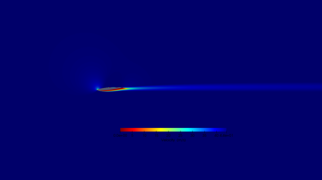
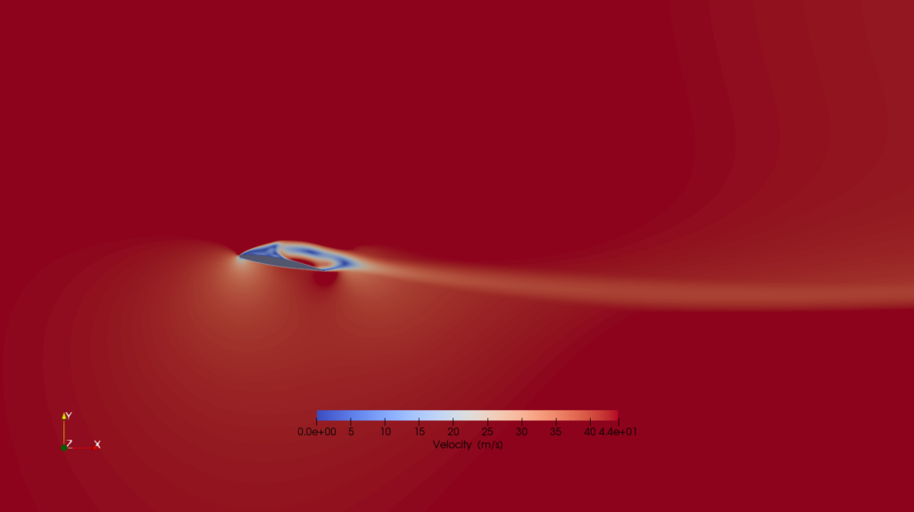
Flow Visualization
Figure 10: Velocity magnitude of flow over the airfoil at angle of attack of negative five degrees
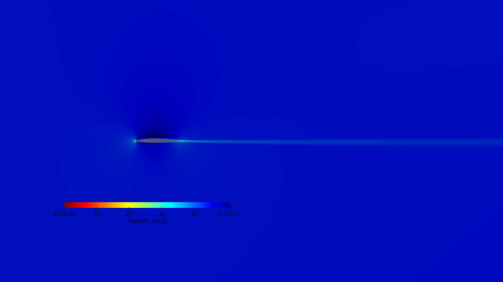
Figure 11: Velocity magnitude of flow over the airfoil at angle of attack of zero degrees
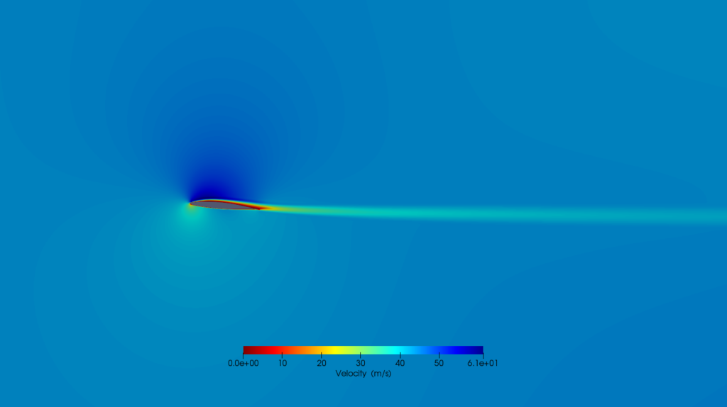
Figure 12: Velocity magnitude of flow over the airfoil at angle of attack of five degrees
Figure 13: Velocity magnitude of flow over the airfoil at angle of attack of ten degrees