“This work would not have been possible without the incentive and contributions made by our project sponsors, Dr. Paul Ziadé and Dr. Christopher Morton, from the Department of Mechanical and Manufacturing Engineering at the University of Calgary.”
Please note that this page lists a brief summary of the actual work done throughout this project. The complete project report can be downloaded by clicking the download button below.
Minimization of Flow-Induced Vibrations Using CFD & Machine Learning
The focus of this project is to minimize flow-induced load fluctuations on a cylindrical bluff body at Re =150 by performing flow control through the positioning of a second cylinder downstream of the flow. The control cylinder’s position will be determined utilizing machine learning methods which are trained using data obtained from a series of validated Computation Fluid Dynamics (CFD) simulations.
In order to quantify the effect of the control cylinder on the flow, a performance metric must be defined. The fluctuating components of the lift can be directly associated with the vortex shedding since the lift arises from the difference in the fluctuating pressure distribution between the upper and lower sides of the cylinder. Therefore, an adequate performance metric for measuring the relative magnitude of vibration would be to measure the main cylinder’s Root Mean Square Lift Coefficient. (CL,RMS).
Development Strategies:
To complete this project the team split the work across two stages over 8-month.
In Stage I, the team focused on performing a significant part of the research required for the solution of the problem to start being developed, which involved investigating the mechanism of flow control that is going to be utilized, the fundamentals of numerical simulations in fluid mechanics, and the algorithms that were used to create low-order models of the flow in the simulations. The research allowed for adequate use of low-level simulation software (OpenFOAM), which provided flexibility with the simulations. The simulations were validated through multiple forms of comparison to published results (Drag coefficient, vortex shedding frequency), and Proper Orthogonal Decomposition (POD) was used to create the low-order representations of the flow in the simulations.
In Stage II, the team will select an appropriate machine learning method to process the library of low-order models developed for the flows corresponding to different control cylinder positions. It is anticipated that a neural network will be used, and if that is the case stage, II will consist of designing the architecture of the network, and training and testing it. The successful development of the data-processing algorithm in Stage II shall result in a generalizable form of predicting the effect of the presence of a control cylinder in the flow, which is expected to be quite a novel accomplishment.
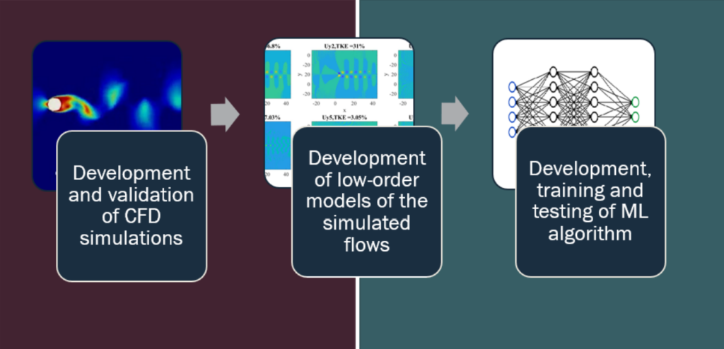
Figure 1 illustrates the major development stages of the project.
Figure 1: Schematic representation of the development stages of the project. (Red side represents stage I and Blue side represents stage II)
Background Research
Strykowski and Sreenivasan's paper in 1990
Before implementing any form of flow control, it was essential to understand the physical mechanism of vortex shedding. As outlined in a research paper published by Strykowski and Sreenivasan in 1990, the vorticities being produced by the flow past a bluff body will diffuse merely through viscus diffusion, and when a certain Reynolds Number is reached, viscous diffusion alone will not be able to diffuse all the produced vorticities. This results in vorticities breaking away at a regular interval and causing vortex shedding. Figure 2 depicts Von Kármán vortices being formed at a regular period behind a cylinder of diameter D. It was found in this same research paper, that the effect of vortex shedding around a circular cylinder could be suppressed at a variety of Reynolds numbers through the correct placement of a smaller secondary body in the wake of the main cylinder. This is particularly important because it demonstrates that upstream flow behavior can be affected by changes made downstream of the flow. Figure 3 depicts vortex shedding suppression through the use of a control cylinder.
Figure 2: Von Kármán vortex shedding at a Re=90 in the wake of a circular cylinder with diameter of D
Figure 3: Vortex shedding suppression using a control cylinder in the near wake section of the main cylinder
Data-Driven Science & Engineering- Singular Value Decomposition
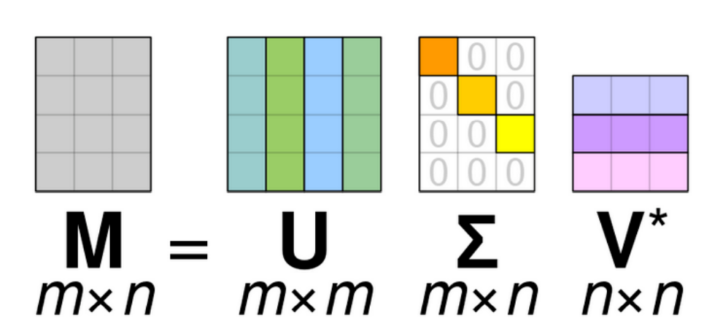
In order to predict an optimal control cylinder position from traditional methods of control, a mathematical model of the system would be required, and generating a model for an unsteady flow with non-linear dynamics and several degrees of freedom is not feasible. The complexity of the problem motivated the use of data-driven methods of control instead of the traditional model-based approach. Several new concepts had to be learned or reviewed, and the work of Dr. Brunton was of great value in the development of the project. The main algorithm utilized in this project and in the next major piece of research is called Singular Value Decomposition (SVD), and a brief description of the algorithm is provided here to enable the reader to follow along with the work that has been done. The SVD is a matrix factorization algorithm that provides a systematic way to determine a low-dimensional approximation to high-dimensional data in terms of dominant patterns. The SVD is guaranteed to exist for any matrix, and it essentially provides a hierarchical representation of the data in terms of dominant correlations. In the interest of keeping this section concise, and maintaining the focus of this report on the project itself, the algorithm will not be explained in depth but instead represented in a way that it could be explained conceptually. A schematic representation of the SVD of a matrix M is represented in figure 4.
Figure 4: Schematic representation of the matrices that result from the Singular Value Decomposition (SVD) of a matrix M
Understanding the meaning of these terms is essential in comprehending how the flow control problem will be dealt with, so the meaning of each of these terms in the context of this project is defined here. M – M is a matrix whose columns represent the entire scalar field of a simulation domain at an instant in time. Picture assembling a scalar field into a very tall, “skinny”, vector for every instant in time, then constructing a matrix whose columns are these vectors, that is M. In two dimensions, M could be a matrix of kinematic pressure (P), x-velocity (Ux), or y-velocity (Uy).
U – U is a matrix that encodes the spatial dependence of the flow, and each column of U can be thought of as a “basis flow”, similar to how in cartesian space the idea of basis vectors is used. Each column of U represents a spatial basis that remains constant in time.
∑ – Sigma is a diagonal matrix containing singular values, which encode the hierarchical relationship between columns of U, making the first basis flow capture more of the spatial variation than the second, the second capture more than the third, and so on.
V* – V* is a matrix that encodes the temporal dependence of the flow, and each row of V* contains the coefficients associated with one of the spatial modes at every instant in time. In order to reconstruct the flow field at an instant in time, the first N modes must be paired with their corresponding coefficients at that time and added together.
What the SVD essentially accomplished in this application is a separation of the spatial and temporal dependence of the flow with the spatial terms being organized in hierarchical order. With this algorithm, a complex flow can be represented at any given instant in time with a linear combination of the first N basis flows and their respective coefficients corresponding to that instant in time.
An Introduction to Computational Fluid Dynamics (Versteeg)
In order to collect data for analysis and training of the neural network algorithm, numerical simulations are used to model and recreate the flow field around the two cylinders. This flow field data can then be extracted and used as the raw data for future analysis. However, to be able to construct such numerical simulation one must have a good understanding of Computational Fluid Dynamics (CFD). To gain the required level of knowledge a book on CFD written by Versteeg and Malalasekera was studied. Majority of the real-life problems that an engineer faces are non-linear. Sometimes these nonlinear problems can be modeled to a high degree of accuracy with a linear model. A great example of this is the spring force equation. Springs inherently behave nonlinearly, but the majority of their characteristics such as the spring force can be modeled using linear equations. Unfortunately, many of the problems faced in the field of fluid mechanics are nonlinear. Furthermore, a linear approximation of these equations would yield incorrect results. For example, The second term on the left-hand side of the Navier-Stokes equations is called the convective flux. This term represents the change in momentum of the fluid due to the unsteadiness of the fluid flow and its convection. This term is highly nonlinear and is mainly responsible for the turbulence in the flow. Approximating this term with a linear equation would yield bad results.
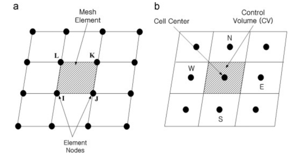
Staying with the nonlinear equations would cause a second problem, it is significantly more complex to construct solutions for these types of equations. However, there are a few workarounds that can help scientists to find a good approximate solution instead of the actual solution, one of which is a numerical approximation. This method uses numerical methods to approximate the governing equations of the flow. Although there are many different numerical methods that can be used, our simulation will use the Finite Volume Method (FVM) to solve the governing equations of motion for the fluid. To use the FVM one must first discretize the flow field which is a continuum, into a finite number of elements. Later the integral form of the conservation equations can be applied to each individual cell in the mesh. Finally, the integrals are replaced with the cell average quantities and the value of the unknown parameters (for example velocity) can be calculated. Figure 5, depicts a continuum being discretized into individual meshes.
Figure 5: Approximation of a continuum using discrete number of meshes
CFD Mesh Refinement
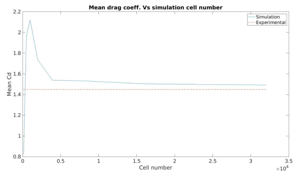
The accuracy of the simulation relies strongly on the mesh resolution. It is important to make sure that the mesh resolution is not influencing the simulation results. There are two methods that could be used for mesh refinement analysis. First, one could track a specific value in the simulation (such as drag coefficient) as the number of cells in the domain are increases. As one can see from figure 10, the drag coefficient starts to approach a constant value asymptotically when the number of cells is increased.
Figure 6: Mean drag as a function of cell number
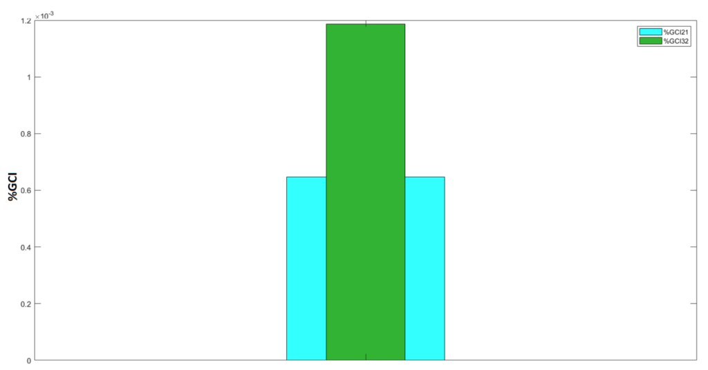
The first method works, but to get better accuracy one must run simulations at high cell numbers. This suggests that the computational cost of running a single simulation would increase. To bypass this problem the method of Grid Convergence Index (GCI) could be used. The GCI is a measure of the percentage, the computed value is away from the asymptotic value. In simple terminology, it indicates how far the solution of the simulation is from the true (asymptotic) value. To conduct a GCI, one must create three different meshes for the same problem. These meshes are all identical in geometry, but they have different resolutions. For example, the coarsest mesh could have 1000 cells then the medium mesh would have 4000 cells and the fine mesh would have 16000 cells. It is important to note that the mesh resolutions must be increased by a constant factor and should not be a random number. The technique uses a set of mathematical equations to calculate the percent difference between the solution and the asymptotic value. Figure 11 shows the GCI conducted on one of the double cylinder simulations. Furthermore, table 1 shows the data used to run the GCI algorithm on.
Figure 7: Percent GCI conducted on the data provided in table 1
Table 1: CFD data used for GCI and Richardson extrapolation calculations.
Mesh Type
Fine
Medium
Coarse
Number of Cells
91827
48845
25058
RMS Drag Coefficient
1.3918
1.3912
1.3923
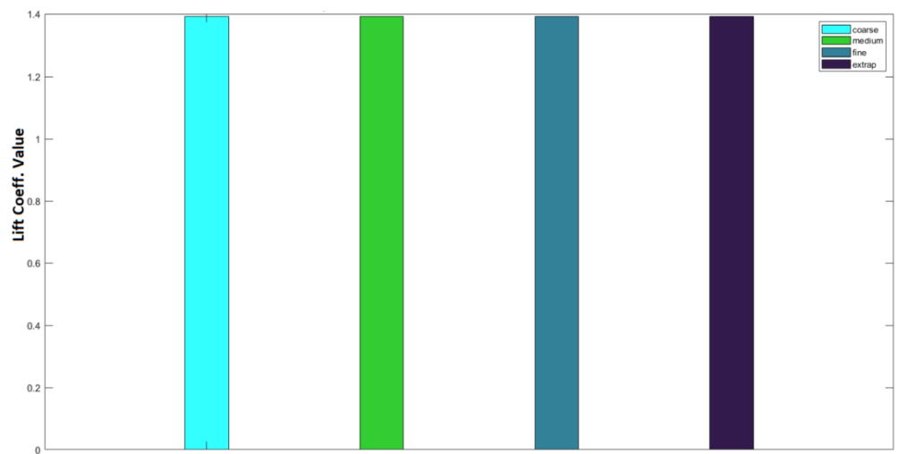
To further validate the mesh resolution a Richardson extrapolation can be conducted. Richardson extrapolation is a method for obtaining a high-order estimate of a continuum value from a series of low-order discrete values. In simple terminology, it is a technique that gives the user the ability to approximate a continuum (no mesh) using a few values obtained through field discretization.
Figure 8: Richardson extrapolation of lift coefficient data for a double cylinder simulation.
To reduce the work needed for creating this website I have decided to end the page here. However, all the details and the results on the performance of the neural network and the construction of the meshes are provided in the full report. The full report can be downloaded from the link at the top of this page.